Pressure Coefficient Measurement in CFD for Wind Engineering

Surface pressure coefficients are the primary output of any wind engineering Computational Fluid Dynamics (CFD) study - every facade cladding check, structural load envelope, and code compliance calculation depends on reliable $c_p$ data. Extracting them from a simulation seems straightforward: take surface pressure, subtract a free-stream reference, normalize by dynamic pressure. The formula matches wind tunnel practice exactly.

The error most CFD implementations make is treating the free-stream reference as a constant. In steady Reynolds-Averaged Navier-Stokes (RANS) analysis, that is correct by construction. In Large Eddy Simulation (LES) and LBM, it leaves low-frequency pressure waves - coherent across the domain but unrelated to the building's local aerodynamics - embedded in every surface probe, corrupting the RMS values and peak statistics that wind codes require.

Why $p_\infty$ Must Be a Time Series

The instantaneous pressure coefficient is:

where $p(t)$ is the surface pressure, $p_\infty(t)$ is the free-stream static pressure at the reference location, and $q = \tfrac{1}{2}\rho\,U_H^2$ is the dynamic pressure based on the mean velocity $U_H$ at the height of interest. The dynamic pressure uses time-averaged quantities and is constant throughout the analysis. Both pressure terms are time series. The subtraction must happen at each time step independently.

Low-frequency pressure waves can appear in the simulation domain from various sources - domain boundary conditions, inflow generation, or large-scale pressure gradients unrelated to the building itself. These waves propagate through the entire domain and are therefore present both at the building surface and at the free-stream reference location. They are not local phenomena tied to the building's aerodynamics; they appear uniformly across the domain.

When the reference is replaced by its time mean $\bar{p}_\infty$, the residual at each instant is:

This residual represents the low-frequency wave at that moment. Because it is present at the reference location but not subtracted from the surface pressures, it enters every surface probe simultaneously. The result is an artificial inflation of the $c_p$ RMS across the full building envelope - not from anything the building is doing aerodynamically, but from a domain-wide signal that does not reflect local pressure fluctuations on the facade. Using $p_\infty(t)$ as a time series subtracts this coherent component at each instant, leaving only the pressure fluctuations that are genuinely associated with the building's flow field. Peak $c_p$ values, which drive facade cladding and structural load design in wind codes, depend on this correction being applied.

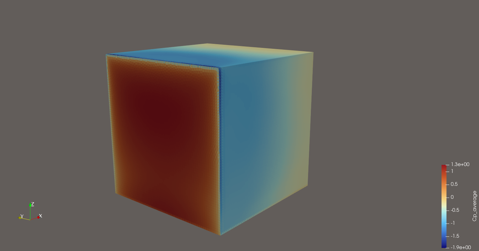
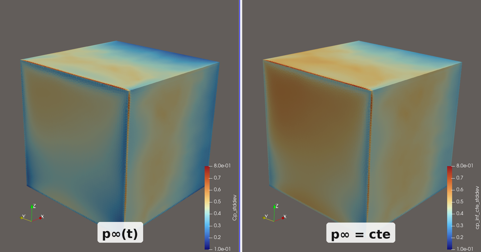
The figure below shows the same simulation processed both ways. The left panel uses $p_\infty(t)$ as a time series; the right uses the time mean. The RMS inflation is visible across the entire surface.

Getting $p_\infty(t)$ Right: Reference Placement

Since $p_\infty(t)$ must be a time series, the reference probe needs to capture the instantaneous atmospheric static pressure - the pressure the flow would have at that location without the building present. Two requirements follow:

• Height: at least $\max(2H,\,400\,\text{m})$ above the roof, where $H$ is the building height. Flow separation over the roof and the stagnation zone above create a pressure disturbance that extends several building heights upward. The reference must sit above this zone.
• Horizontal position: directly above the building centroid, or far enough laterally that blockage effects are negligible.

If the probe sits within the building's pressure influence zone, the building's own field contaminates $p_\infty(t)$ and biases every $c_p$ value. The $\max(2H,\,400\,\text{m})$ rule is a minimum - terrain or dense surroundings may require moving the probe further.

Both the body surface export and the reference point export must share the same time range and sampling interval. A timestep mismatch makes the per-instant subtraction impossible.

Getting $p(t)$ Right: IBM Offset

Correct reference subtraction depends equally on a clean surface pressure signal. In a Lattice Boltzmann Method (LBM) solver using the Immersed Boundary Method (IBM), geometry is represented as an STL surface mesh, with one Lagrangian point placed at each triangle centroid. No volume mesh is generated. The IBM enforces the no-slip condition by exchanging forces between these Lagrangian points and the surrounding fluid lattice.

This introduces a near-wall zone - roughly $1.5$ lattice cells from the surface - where pressure is influenced by the IBM interpolation and force-spreading kernels rather than being fully resolved by the LBM stencil. Sampling at the geometry surface returns values partially contaminated by numerical artifacts.

The fix is to set normal_offset = 2 * body_ref in the body export configuration, where body_ref is the lattice resolution assigned to the geometry in meters. This displaces every probe two lattice cells outward along the surface normal, placing all sampling points in the fully resolved fluid region. For a body refined to $\Delta x = 0.5\,\text{m}$, normal_offset $= 1.0\,\text{m}$.

Computing $c_p$

After the simulation, a short Python script performs the subtraction. It loads the reference pressure time series, computes $c_p$ for every surface triangle at every timestep, and writes the result into the body HDF5 file as a new cp/ group. The script also patches the XDMF descriptor so the $c_p$ field appears immediately in ParaView. The core computation is:

cp = (p - p_inf[key]) / q

The script validates that body and reference files share identical timestep keys before proceeding. Dependencies are h5py and numpy only.

What Correct $c_p$ Enables

Once the time-synchronized subtraction is applied correctly, the $c_p$ time series supports the full range of wind engineering analysis: mean and peak $c_p$ maps, RMS distributions for fatigue assessment, and structural load integration. LES resolves the transient pressure fluctuations - vortex shedding, separation bubbles, reattachment zones - that RANS structurally cannot provide. But those physics are only accessible if the post-processing methodology matches the physics: a time-varying reference for a time-varying simulation.

The full configuration details - body export setup, reference point positioning, and the Python script - are in the pressure coefficient measurement guidelines.