Atmospheric Boundary Layer Simulation: From Setup to Validation

Wind load analysis, pedestrian comfort studies, and urban wind assessments all share a common prerequisite: a well-characterized Atmospheric Boundary Layer (ABL) profile. Get the inlet wrong, and every downstream result inherits that error. Yet in practice, generating and maintaining a consistent ABL across a long simulation domain remains one of the more frustrating steps in a Computational Fluid Dynamics (CFD) workflow - with the mean velocity and turbulence intensity profiles tending to decay well before reaching the building of interest.

The standalone ABL simulation is the first validation step in any wind engineering CFD study: an empty-domain run that confirms the wind profile at the region of interest matches the target terrain category before any geometry is introduced.

Why a Standalone ABL Case?

The standalone ABL case is a rectangular domain with no buildings or obstacles. Its only purpose is to verify that the turbulent inflow conditions prescribed at the inlet are faithfully transported to the measurement section. Once validated, the entire configuration - roughness elements, inlet parameters, domain height - transfers directly into the production simulation with buildings or terrain.

This is standard practice in wind tunnel testing (the empty-tunnel profile check) and should be standard practice in CFD as well.

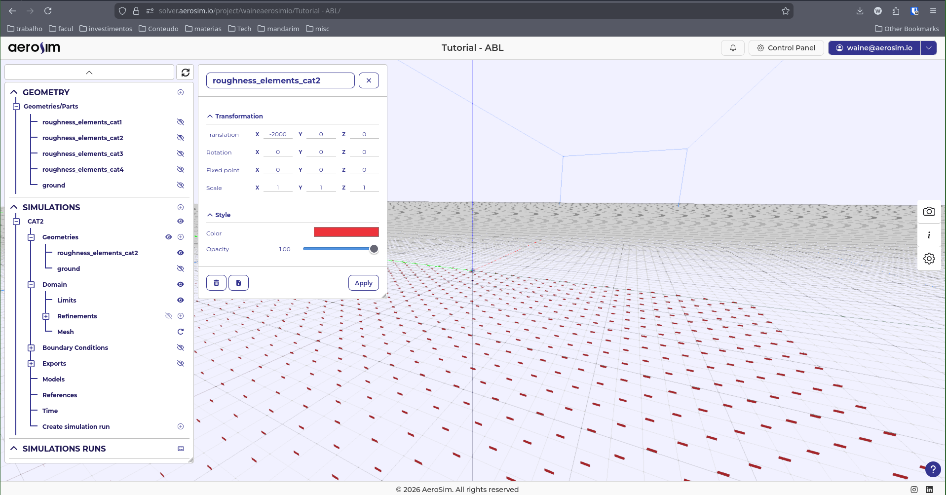
Domain and Roughness Elements

AeroSim's Lattice Boltzmann Method (LBM) solver achieves roughly $10\,\text{M nodes/GB}$ of GPU memory, which means large domains do not require proportionally large hardware. The reference ABL case uses a domain of $7200\,\text{m} \times 2000\,\text{m} \times 1000\,\text{m}$ (streamwise, cross-wind, height).

The domain is translated so the region of interest sits at $x = 0$, with a development length of $1500\,\text{m}$ upstream. This fetch allows the synthetic turbulence injected at the inlet to reorganize into a physically consistent state - visible when the energy spectrum recovers the $-5/3$ inertial subrange at the measurement section.

Physical roughness elements - arrays of solid fins on the ground surface - generate and sustain the turbulent shear layer. Fin height is calibrated per terrain category according to EN 1991-1-4. For terrain category II ($z_0 = 0.05\,\text{m}$), the fins are $2\,\text{m}$ tall, spaced on a $16\,\text{m} \times 32\,\text{m}$ grid. Because AeroSim uses the Immersed Boundary Method (IBM), these elements are simply imported as STL files - no volume meshing required.

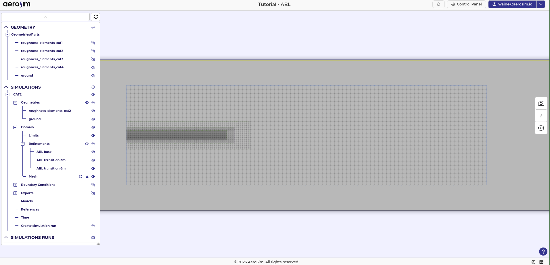
Mesh Refinement

Starting from a $10\,\text{m}$ baseline resolution, three levels of octree refinement bring the near-ground cell size down to $1.25\,\text{m}$. Three nested refinement boxes concentrate resolution where it matters:

• ABL base: $1.5\,\text{m}$ target, extending from the inlet to $500\,\text{m}$ downstream of the region of interest, up to $80\,\text{m}$ height.
• Two transition layers at $3\,\text{m}$ and $6\,\text{m}$ target resolution, providing smooth cell-size transitions to the baseline.

The final mesh contains approximately $47\,\text{M}$ nodes and requires about $5\,\text{GB}$ of GPU memory - comfortably within the range of a single workstation GPU.

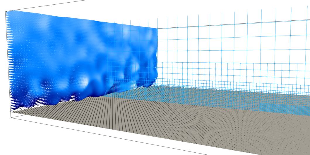
SEM Inlet Generation

The Synthetic Eddy Method (SEM) is the core of AeroSim's turbulent inflow. Rather than imposing a frozen velocity profile at the inlet, SEM distributes $N$ synthetic eddies in a virtual volume around the inlet plane. Each eddy carries a Gaussian influence function and random orientation signs. The resulting velocity field at the inlet is:

where the fluctuation $u'_\alpha$ is constructed so that its time-averaged statistics converge to the prescribed Reynolds stress tensor $R_{\alpha\beta}(z)$. The fluctuations are computed via the Cholesky decomposition of $R_{\alpha\beta}$, which ensures correct cross-correlations between velocity components.

In practice, the setup is straightforward. AeroSim includes an automatic profile generator: given the reference wind speed ($U_{ref} = 20\,\text{m/s}$ at $z_{ref} = 10\,\text{m}$ for this case), it constructs the mean velocity and Reynolds stress profiles from standard analytical models. Three inputs in the interface - roughness length, target velocity, and reference height - replace what would otherwise be a manual CSV file with eight columns of profile data.

Consistency Matters

One critical requirement: the SEM inlet profile and the ground boundary condition must use the same roughness length $z_0$. If they are inconsistent, the velocity profile drifts as the ground boundary layer adjusts to the actual floor roughness. AeroSim's ground boundary condition uses an equilibrium log-law wall model (ABL Wall Model) that takes $z_0$ as a direct parameter, making consistency easy to verify.

Solver Settings

The turbulence model is Large Eddy Simulation (LES) with the Smagorinsky subgrid model ($C_S = 0.17$). The simulation runs for $720\,\text{s}$: the first $120\,\text{s}$ are discarded as flow development, leaving $600\,\text{s}$ for statistics. The time step $\Delta t = 0.032\,\text{s}$ corresponds to a CFL of $0.1$, keeping the lattice Mach number well below the stability limit of the weakly compressible LBM formulation.

The dynamic viscosity is chosen to target $Re = 10^5$ rather than the physical air value. Full-scale ABL flows operate at $Re \sim 10^8$, which is impractical to resolve directly. The standard LES practice is to select a moderate Reynolds number that maintains fully turbulent flow while keeping viscous effects negligible at resolved scales.

For a full walkthrough of the case setup - including boundary condition parameters, refinement configuration, and solver controls - see the ABL guided case in the documentation.

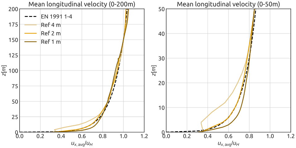
Validation Workflow

A vertical profile line at $x = 0$ (the start of the region of interest) samples velocity from ground level to $200\,\text{m}$, every $0.1\,\text{s}$ from $t = 120\,\text{s}$ onward. This provides both time-averaged profiles and sufficient temporal resolution for frequency spectra.

Some validation checks are:

1. Mean velocity $U(z)$: the simulated profile at the measurement section should match the target log-law within $\pm 10\%$ across the height range of engineering interest.
2. Turbulence intensity $I_u(z) = \sigma_u / U(z)$: compared against the target profile from the applicable wind standard (EN 1991-1-4, ASCE 7, or similar).
3. Profile maintenance: the profiles should be sustained across the region of interest, confirming that the combination of SEM inlet and roughness elements prevents the profile decay.

Quantitative validation results - including velocity, turbulence intensity, integral length scale, and energy spectra comparisons - are available in AeroSim's validation portfolio.

Key Takeaway

The ABL case reduces to a small number of physical inputs - terrain category, reference wind speed, roughness length - and a domain sizing exercise. The SEM inlet eliminates the need for precursor simulations or recycling methods, and the IBM treatment of roughness elements removes volume meshing from the workflow entirely. With a ~50M node domain running on a single GPU, this is a validation step that can (and should) precede every wind engineering simulation.